An analysis of Oakland Crime 2007-2012

1 Nov 2013

With the help of OPD, I have collected public data regarding almost 400,000 Oakland crimes for the years 2007-2012, and classified these into a hierarchic set of “crime types,” e.g.:

• LARCENY

  • LARCENY_BURGLARY

    • LARCENY_BURGLARY_AUTO

    • LARCENY_BURGLARY_COMMERCIAL

    • LARCENY_BURGLARY_OTHER

    • LARCENY_BURGLARY_RESIDENTIAL

The simplest analysis combines data across the years 2007-2012¹ and considers each beat’s pattern across a subset of the most common crime types. The second question considered is how these patterns have changed over the last two years (2011, 2012): is a particular category of crime going up/down during 2011-2012 relative to the six year average?²

A high standard is used to highlight 2011-2012 changes: Only when a beat’s totals for both 2011 and 2012 were significantly above/below the
beat’s historical average is it reported. Further details are also available:

• Construction of the data set

• the OakCC  crime classification

Here’s an example: there were 7878 ROBBERY_FIREARM crimes during 2007-2012 across all of Oakland, working out to an average of 138 per beat. 88 of these occurred in Beat 18X, significantly lower than the city-wide average; it’s Z-score is -4.68. Considering all six years of 2007-2012, this beat’s 88 ROBBERY_FIREARM makes for an annual average of 14.67. But in fact 23 ROBBERY_FIREARM occurred in 18X in 2011 and 24 in 2012, both much above 18X’s annual average, and so this change is considered significant.

You can’t see it from any one beat’s report, but there are also important similarities between the beats, in terms of common patterns of the types of crimes they experience. That is, while the dominant crime types in some beats are LARCENY_BURGLARY_AUTO, LARCENY_BURGLARY_RESIDENTIAL and ASSAULT_FIREARM; the patterns of crime are correlated. In other beats the dominant crime types are DOM-VIOL, LARCENY_THEFT_GRAND, COURT, LARCENY_THEFT_VEHICLE_AUTO, ROBBERY and SEX_PROSTITUTION. Finding patterns in these correlations across beats
is difficult; here are three ways to visualize them.

The first figure  shows the beats as a graph:

Connecting similar beats

Dots/nodes correspond to different beats, and an edge connects two
nodes if their patterns of crime are highly correlated. The nodes
have also been colored by their City Council district. Focusing on
the cluster of nodes in the upper left corner, it’s interesting to
note that these crime-similar beats fall across multiple
geographically distributed districts.

A second way to visualize inter-beat similarities relies on a more complicated statistical trick called “dimensionality reduction.” The basic idea is that rather than treating each crime type as independent, we can “collapse” those that occur in similar patterns across beats and merge them into a single “super” crime type. The second figure uses these tricks to display all the beats in terms of two such super-crime-types, corresponding to the horizontal and vertical axes. The important
feature of such visualizations is that beats with similar patterns
of crime are plotted close to one another. Not all beats have
been labeled here (it gets too crowded!), but again you can see that
beats with similar crime patterns come from across geographic districts.

Two dominant dimensions of crime type variability

Finally, if we consider just a single, most important of the super-crime-types (corresponding to the horizontal axis in the figure above) we can use it as a scale to rank all beats. Being very negative on this scale means that a beat experiences lots of DOM-VIOL, LARCENY_THEFT_GRAND, COURT, LARCENY_THEFT_VEHICLE_AUTO, ROBBERY and SEX_PROSTITUTION, while being very high on this scale means that a beat instead experiences primarily LARCENY_BURGLARY_AUTO, LARCENY_BURGLARY_RESIDENTIAL and ASSAULT_FIREARM. The scale can then be used to color a map of Oakland’s beats, and that is the third figure. Geographic variation in crime types is especially obvious in this map.

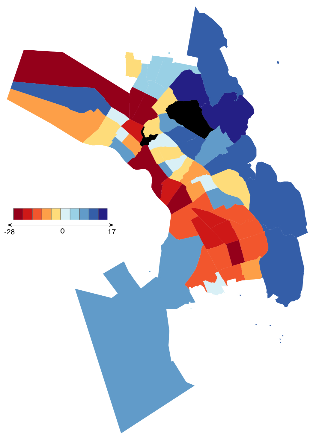
Beats as they vary with respect to the biggest dimension of variability